Calculate Ratio with GCD
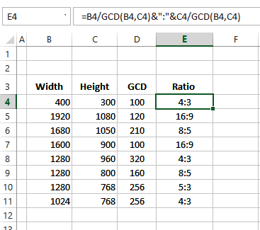
In this example, there is a list of screen dimensions, with the first width — 400 — in cell B4 and the first height — 300 –in cell C4.
To calculate the ratio for each screen, the formula will use the GCD function, which returns the Greatest Common Divisor, for two or more numbers.
NOTE: In Excel 2003 and earlier, the Analysis Toolpak must be installed, to use the GCD function.
Test the GCD Function
To see the largest number which will divide equally into the numbers in B4 and C4, enter this formula in cell D4:
=GCD(B4,C4)
The result is 100.
Create the Ratio Formula
To calculate the ratio, the width will be divided by the GCD and the height will be divided by the GCD. A colon will be placed between those two numbers.
To see the ratio, enter this formula in cell E4:
=B4/GCD(B4,C4)&”:”&C4/GCD(B4,C4)
The result is 4:3 — the ratio for those screen dimensions.![]()
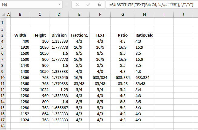
Ratio With TEXT and SUBSTITUTE
Another way to calculate ratio is with the TEXT and SUBSTITUTE functions — these functions work in all versions of Excel, without the Analysis Tookpak having to be installed.
In this example, there is a list of screen dimensions, with the first width — 400 — in cell B4 and the first height — 300 –in cell C4.
To calculate the ratio for each screen, the formula will divide the width by the height, and format the result as a fraction. Then, the slash will be replaced with a colon, to create the ratio.
Test the TEXT Function
To see the result as a fraction, enter this formula in cell D4:
=TEXT(B4/C4,”#/######”)
The result is 4/3.
Create the Ratio Formula
To calculate the ratio, the width will be divided by the height, and formatted as a fraction. A colon will replace the slash.
To see the ratio, enter this formula in cell E4:
=SUBSTITUTE(TEXT(B4/C4,”#/######”),”/”,”:”)
The result is 4:3 — the ratio for those screen dimensions.